In today’s fast-paced world, people expect to get answers to their queries in a few microseconds. The demand becomes more prominent when organizations maintain many Excel sheets. What if you have to find something in a large spreadsheet and have a tiny piece of information to start?
Here comes the role of VLOOKUP in the frame that can help you search for small and extensive information in Excel spreadsheets when you are always looking for the same data. Using this formula is essential to perform data science processes in Excel.
It matches data across sheets, consolidates information, and generates meaningful insights. It is also helpful in increasing efficiency, reducing errors, and making users make informed decisions by extracting relevant data quickly.
VLOOKUP is essential when used in financial modeling or another type of financial analysis to make models more attractive and incorporate multiple scenarios. For business, research, and finance, VLOOKUP works as a vital formula, catalyzing the transformation of raw data into actionable knowledge with unparalleled speed and precision.
This article will teach us to use VLOOKUP in Excel spreadsheets to get the correct information.
What is VLOOKUP?
VLOOKUP or Vertical Lookup is a function in Excel used to retrieve data from other data sources. It acts like a phonebook on your mobile where you can start searching with a small data piece you know. It can be someone’s name to find out what you don’t know, like their address, phone number, or email address. In short, VLOOKUP is all about summarizing the whole data and saving precious time.
VLOOKUP is a function to find specific information across a table or Excel spreadsheet in a vertical pattern. It makes Excel search for a particular value in a column to find a deal from a different column in the same row. The VLOOKUP tool uses four specific arguments: Lookup Value, Table array, Col index num, and Range lookup.
How to use VLOOKUP in Excel?
In Excel, VLOOKUP helps us look up a piece of information in a table or data set to get some correlated data or information. The VLOOKUP tool says to Excel,” Look for the piece of information (for example, an apple) in this data set (a table) and tell me something more related to it (for example, the price of apples). Here are some essential steps to use VLOOKUP in Excel.
Syntax
The syntax or formula for the VLOOKUP function is typed as:
=VLOOKUP(lookup_value, table_array, col_index_num, [range_lookup])
In above- mentioned four specific features, VLOOKUP takes these parameters:
Lookup_value: Select the cell or column where the search values that should be in the first column of the table will be entered.
Table_array: Enter the cell’s range containing the data and ensure the first column holds the lookup values.
Col_index_num: It is the data that is being searched or looked up. The input should be the column number, counted from the left. For example, the first column in the following table is 1.
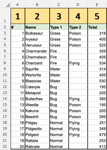
Range_lookup: Optional. If TRUE (or omitted), it searches for an approximate match. If FALSE, it searches for an exact match. Simply, if the number is 1, it means TRUE, and if the number is 0, it is FALSE.
Key Points to be Noted
- Various parts of the function are separated by a symbol, like a comma or semicolon.
The symbol depends on your Language Settings.
- Both 1 / 0 as well as True / False can be used in Range_lookup.
Let us understand it with the following example:
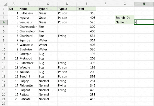
Step by step, type the following instructions:
- Select a cell of your choice (H4)
- Type =VLOOKUP
- Double-click the VLOOKUP command
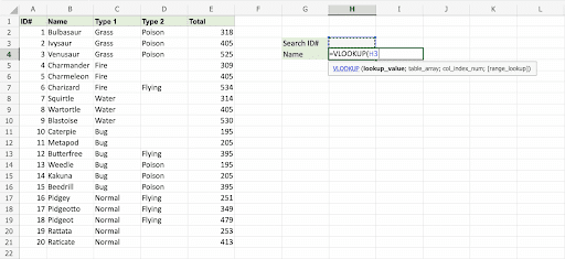
- Now select the cell where the search value is going to be entered (H3)
- Type comma (,)
- Mark the table range ( A2:E21 )
- Again, type comma (,)
- Type the number of the column, counted from the left (2)
- Type 1( TRUE) or 0 (FALSE) (1)
It will look like : =VLOOKUP(H4, A2:E21, 2, TRUE)
- Press the Enter key for executing the formula
- After that, enter a value in the cell selected for the Lookup_value H3 (7)
Select the Result Cell
Now, you click on the cell where you want search results to appear after applying the VLOOKUP function.
H4 is where the search result is displayed. In this case, the names are based on their ID#.
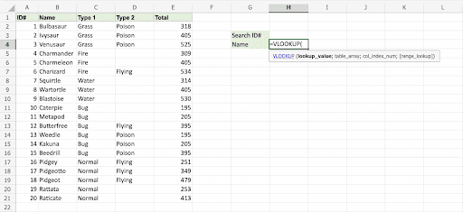
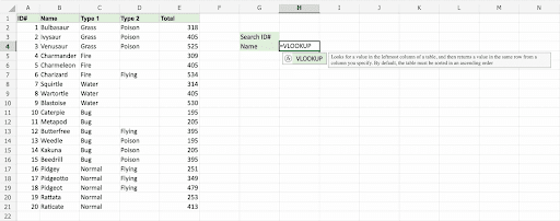
We have selected H3 as a lookup_value. It is the cell where the search information is entered; in this case, the given ID #
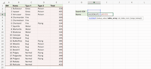
The table range is marked at table_array; so in this example, it is A2:E21.
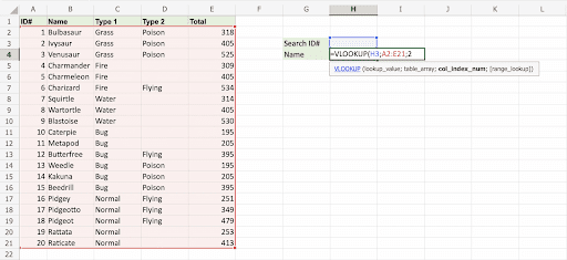
Here, number 2 is entered as col_index_number. It is the second column from the left and the date being searched for.
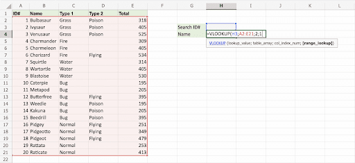
Further, here is an example of selecting col_index_number 2.
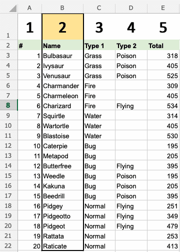
Next – 1 (True) is entered as range_lookup. This is because the left column has only numbers. If it was text, 0 (False) would have been used.
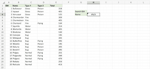
The function returns the #N/A value. No value has yet been entered into Search ID# H3. Now we feed a deal to it, type H3 ( 7):
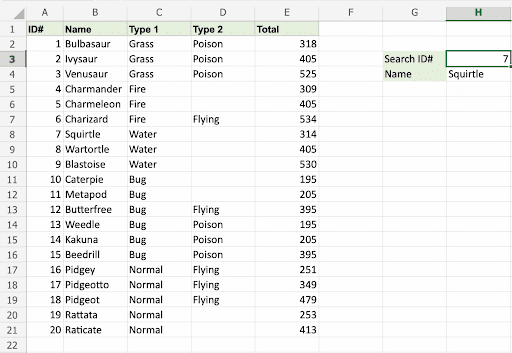
Finally, the LOOKUP function found the ‘Squirtle’ with ID# 7.
Again type (H3)4:
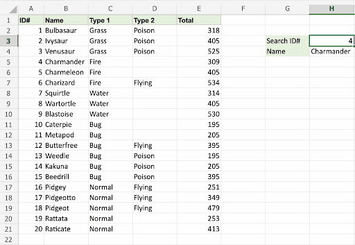
As a result, the function returned the Charmander name, which has four as its ID#.
This is how we can use the VLOOKUP function in Excel.
Bottom Line
So we have seen steps of using Vlookup in Excel, but there are a few things to be kept in mind like the VLOOKUP function can not look at its left and searches in the leftmost column of the table array and provide a value from a column to the right. This function is case-insensitive, and lowercase and uppercase characters are treated as equivalent.
Using TRUE or FALSE for full details is essential and should be considered. In this function, the data in the lookup column should be stored in ascending order. With these steps and guidelines, one can easily use the VLOOKUP function in Excel and find the appropriate information with less effort.
Welcome to our blog! My name is Yuvraj Kore, and I am a blogger who has been exploring the world of blogging since 2017. It all started back in 2014 when I attended a digital marketing program at college and learned about the intriguing world of blogging.


